By: Vladimir Ivanov
- Scope
- Definitions & Overview
- Artificial Neural Networks
- The Multilayer Perceptron
- Training
- But why ?
- Implementing a Neural Network from scratch (with numpy)
- The Basics: Overview of Linear Regression
- Gradient Descent
- Neural Networks
- A generalized implementation of a Neural Network
- Layers, Training, Backpropagation
- Stochastic Gradient Descent (SGD)
- Improving our implementation.
- The Adam Optimizer
- Hardware acceleration with CUDA & CuPy
- Going further
- Tests & takeaways
The scope of this article is to analyze the implementation of the Multilayer Perceptron algorithm and provide the reader with both an in-depth formal overview of the math that underlay it and also display a practical implementation in Python. The article is lengthy, but is done in a modular way, so a beginner and intermediate readers can both take away something useful from it. After the implementation part, our MLP will be applied to model multiple real-world datasets and evaluated against the MLP algorithm from the most popular, established ML library Tensorflow
Artificial Neural Networks (ANNs) are a type of statistical inference algorithms, loosely based on the real world, biological neural networks[1]. Every ANN has a set of hierarchically connected artificial neurons, that are stacked together in groups (layers).
An Artificial Neuron is a mathematical function or a composition of multiple functions. During inference, every neuron recieves an input signal. The inputs to that neuron are then weighted with by a linear coefficient and afterwards (usually) an activation function is applied.fig 1
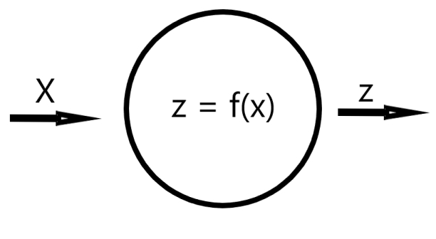 [fig 1]
The input signal is usually a number or a list of numbers, grouped in a vector. The signals travel from the first layer (input layer), they undergo transformations in the hidden layers and then they reach the final (output) layer (fig 2) .
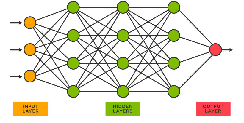 [fig 2]
The algorithm this article will focus on is the Multilayer Perceptron. It is the most basic, "vanilla" class of neural network algorithms. In this article, the terms MLP, NN, Neural Network will be used interchangeably to mean Multilayer Perceptron. Note that MLP is far from being the only type of neural network.
Some types of neural nets, that build upon the understanding of MLPs are:
- Convolutional Neural Network (CNN)
- Recurrent Neural Network
- Graph Neural Network
- ... and lots more
Each of these have many interesting uses, that are unfortunately beyond the scope of this article.
A MLP consists of an input layer, (at least 1) hidden layer and an output layer. Typically MLPs also feature a non-linear activation function for their hidden layers.
Perceptrons can be used for both regression and classification.
Neural networks are trained by processing training examples of a dataset in an attempt to map a set of characteristics (features) to a desired output result. Each training example must therefore contain both features and a result.
During training, the network typically makes a prediction for a training example and then computes an error, measuring how its prediction is off from the actual example result.
For example, if given a function
we ask our network to make a prediction for F(5) and it yields 10, then we compute
This type of error (loss) also has a name. It's called the absolute error, but that will be mentioned later :)
The error is then returned to the layers via a process called 'backpropagation' which will be explained in a later section. During backpropagation, the weights of the layers are adjusted as to minimize the error over the next iteration.
A neural network "learns" a very close approximation of the F function if given a big enough training set and iterated over that set enough times.
Why would we need a complex algorithm for our task when we can deduce that F(x) = 2x + 5, given 3 or 4 values for x? Additionally why only approximate this function when we can know its exact definition. This is a good question, and for functions as simple as our little F example, we should aim to determine the exact function.
Suppose this task however
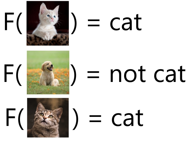
In this example, our X is now an image and our task is to determine whether or not the image is of a cat or not. How would we even begin to approach this task algebraically ?
Here, lets try it. Suppose I is our grayscale matrix representation of the image
Then we can just simply find if
Or if the pixel value for the center pixel is equal to 0 (black) because dogs have black noses. This turned out simpler than we thought, trivial even😎. Now we just need to flip the result and we have a cat classifier. Oh wait..
But what if the nose of the animal isn't on that center pixel. Or what if that pixel is black because of the environment ? Say the cat is laying straight next to it on a black blanket.
Or what if we have to classify a Bombay cat ?
Furthermore, what even is a cat? What ontological qualities must an entity posses in order to be classified a cat? How do we translate the immaterial Platonic form, the ideal of a cat formed throughout our thousand personal experiences of seeing cats, to something we can algorithmically model ?
The answer was in the question :)
Before we dive straight to the 'deep' of deep neural networks, lets first analyze the algorithm that makes everything work with a much simpler problem: Linear Regression.
is a simple algorithm that, just like NNs, is used for statistical inference. The term 'linear' means that the prediction model is going to attempt to fit a linear mathematical function to the set of data points provided. We'll take a look at a simple linear regression type.
A test set of data points (dataset) that is often used as a machine learning benchmark is the famous Boston housing dataset.
For this example however we'll be using a simplified mock dataset with only 1 feature, called the
drumroll
Here is an example of what the records look like:
| Table | Plot |
|---|---|
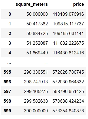 |
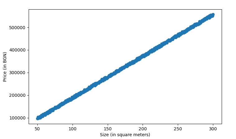 |
We can clearly see that for this dataset, the points follow a linear pattern.
Therefore, there must exist some linear function
That can estimate our little set of points almost perfectly.
To find the values for w and b is where linear regression comes in.
Note that the names w and b are not random and are named after weight and bias.
We can initially randomly set w and b and run inference with each of our samples and store our predictions in a variable
The next step is to find out how far off we are from the actual
There's many ways to do that, but we'll measure it using the mean squared error
Mean squared error is a way for us to quantify the error, made by our little regression model.
Essentialy it takes the mean of the sum of all squared errors between prediction and actual value.
which can be viewed as
We now have a function which quantifies exactly how wrong our model is :)
This is very good, because if we find the parameters w and b, for which L yields a lower value (note that we exclude x and y, since they are constant), we have made an optimization
If we plot the cost function with respect to some random values generated for w and b we can see graphically that there is indeed a place (or a direction), towards which our L function tends to decrease in value
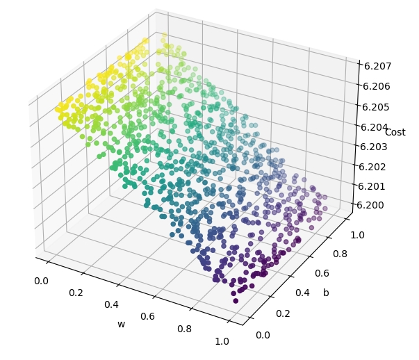
So how do we find the direction in which our L function will decrease in value ?
We can find the function's gradient at a specific point. Or with less mathematical formality, we can find how a change of values for both w and b will affect the loss function value.
To do that, let's first analyze how the loss value is computed.
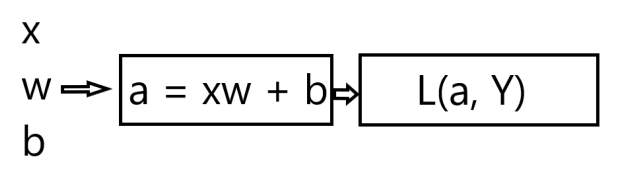
First, for inputs x, w and b, we calculate the value of a with our linear function
Then we pass its output to the loss function.
where a is our prediction for the price of a housing unit and Y is the actual, true price
the error term can also be expressed like this:
Now that we know the chain of computations that need to happen in order to get our loss / error value, we can start computing the gradient.
A gradient of a function for a given point is a vector, with a direction in which the function value increases at the fastest rate. The components of that vector are the partial derivatives of the function with respect to that point and the function input.
So:
Following that we can get :
Which is a gradient vector with 2 components. Expanding on those components we get that:
This is all the math we're going to need to implement linear regression :).
If we had to put all this into an algorithm, it would look like this
We perform N steps, and for each of those steps, we compute dl_dw and dl_db, which are partial derivatives with respect to w and b, for all of the training examples.
The derivatives are multiplied by a constant value alpha (or learning rate), which indicates how big of a gradient step we'll perform
We then subtract the derivatives from the w and b parameters, because by definition:
the direction of the gradient is the direction in which the function increases most quickly
And we want to minimize the value of L, therefore we care about the inverse of the direction of steepest ascent.
This algorithm even has a fancy name. It's called Gradient descent and it is one of the most important and widely used algorithms in modern neural networks.
We can then 'fit' our set of input features to the set of output values and ((( generally ))) if given a large enough N, we should be able to estimate our function quite close to the original.
[Fig 4]
In the Drujba Housing dataset, the original values were generated with
Where
to introduce variance and simulate the imperfectness of real world data.
Our linear regression model, trained with N=50, managed to best estimate the data with
Having gone over this, now its time to go deeper
If we had to define neural networks with what we already know, we'd define them as multiple interdependent regressions on steroids. The 'interdependent' part comes from the fact that the inputs from one layer of little regression units(neurons) come from the output of the previous layer. So can think of each of the neurons[fig 2] of the neural network as a separate regression, where each neuron layer J gets its inputs from J - 1 and outputs its 'activations' to J + 1. But lets not get ahead of ourselves.
How is an algorithm created during WW2 still useful today ?
As explored with the cat example, we (as people) can know for 99.9% certainty that a cat is in fact a cat when we see it. However, how can we translate that to a machine ? Sometimes it is really difficult to put that knowledge into an algorithm and have it make good generalizations.
Other times we have good readable human data, with lots of features, say 10000, but we have no domain knowledge whatsoever about the problem. We don't know which features are useful, which should be combined into a polynomial with others and so on.
If you don't have a domain expert at hand, it is futile to try to model it into a single regression and expect to get good results.
That's where neural networks come in. They allow us to model data with much more complex relationships between X and Y than a line or a polynomial. The algorithm is mysteriously good at finding relationships between input and output data. Too good even, that's why sometimes it is necessary to 'regulate' it, so it makes better generalizations. Hopefully we'll be able to clear some of the mystery as to how it works in the section below :)
Before we start writing python, lets quickly run through all the components of a MLP network.
We must have
- Functionality to define layers
- Layers themselves
- Function to make predictions
- Functionality to train the network
That's all there is to the base MLP algorithm !
And it can be done in less than 100 lines of code **
** If the implementation is case-specific, i.e only supporting a single activation / loss
class NN:
   def __init__(self, layers, loss='mse', optimizer=SGD()):
	self.loss = loss
	self.layers = layers
	self.optimizer = optimizer
	for layer in layers:
	    layer.optimizer = copy.copy(optimizer)
We create a class, called NN and in its constructor we have a layers parameter, which will be used for defining layers, inspired by Tensorflow's sequential model. Additionally, the constructor takes the loss function as a parameter, and as a default we have mse which stands for mean squared error (the one used for our linear regression example).
The optimizer property will be described in detail in the training part
As mentioned above, a semi-accurate way to view a neural network neuron is to view it as a separate regression. And as we saw with the linear regression example, we must have some w and b coefficients, in order to take an input and apply a weighted linear function F
In neural networks, each layer has 1 or more neurons. Each of the singular neurons has its own w and b coefficients and all neurons in a layer share an activation function.
An activation function is a function which processes the weighted input with the goal of introducing non-linearity. If we have an activation G, then it will be applied to our neuron's output as follows:
or
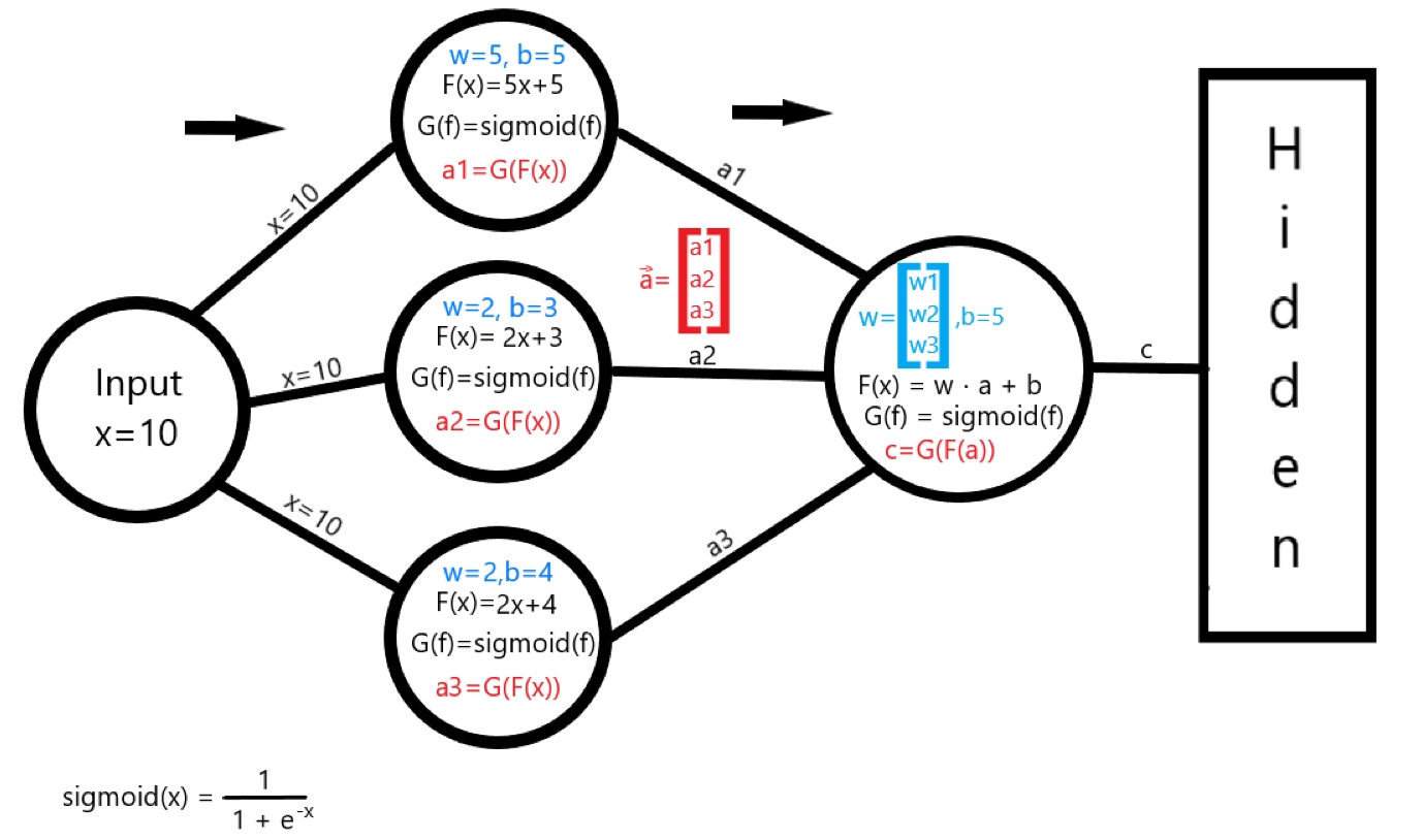
[fig 3]
A simple example of how a neural network transforms an input value through a layer can be seen in [fig 3]
The network has been trained and has found some coefficients w, b (values in blue) for each of the first layer's neurons. Then, the inputs are weighted with the linear function
with each of the neurons' w and b values.
The next step is to compute the activation G, which for this example is the sigmoid activation function
Finally, each neuron computes an activation value Eq 1
Because we have 3 neurons for this layer, the next layer will recieve the activation vector
Following this logic, layer 2 will perform the same operations on a, instead of x, however this time taking the dot product, because a is a vector and so is w
Lets start defining the class
class Layer:
    def  __init__(self, input_size, output_size, activation, kernel_initializer=None):
	self.kernel_initializer = kernel_initializer
	self.optimizer = None
	if kernel_initializer is  None:
	    self.kernel_initializer = XavierInitializer(input_size, output_size)
	self.activation = activation
	self.W = self.kernel_initializer.W()
	self.B = self.kernel_initializer.B()
The class takes in multiple parameters on construction
input_size is the size of activation values from the previous layer (or the amout of features from the input layer)
output_size is the amount of neurons that the layer has.
activation is the activation function for all of the layer's neurons
There are many activation functions that have different applications, but the must-haves are:
ReLU
which is an abbreviation for rectified linear unit. ReLU is super simple, fast and able to achieve non-linearity. It is the most popular choice for a hidden layer's activation.
It is defined as
Sigmoid
The sigmoid activation function is a function that transforms any numeric input from (-∞, ∞) to [0, 1). It is very useful as an output layer activation to predict the probability of a binary classification problem. Its definition is:
Softmax
The softmax activation function converts a vector of K numbers into a probability distribution for K possible outcomes. It is used as a final layer activation of a multi-class classification problem. It is defined as:
and
kernel_initializer is the 'algorithm' by which the weights and biases of the layer will be initialized.
The name 'kernel' simply means matrix. Every layer has w and b matrices, instead of storing the w and b values as vectors per neuron. This is done in order to greatly speed up the training process.
Depending on the layer's activation function and the overall architecture of the neural network, there could be advantages of initializing the weights and biases differently. For most cases it is enough to use the default, Xavier Initialization
Xavier initialization works by randomly initializing the weights using a gaussian distribution, defined as
And
Where i is input_size and o is output_size
The next step is to enable the activation pass and the weighted linear pass of the data.
We define 3 functions:
- dense_pass(X) is responsible for applying a linear weighted pass of the raw X data.
- activation_pass(X) takes the output of the dense_pass function and applies a non-linear (or linear) activation function.
- layer(X) combines the two together as in Eq 1. Additionally it caches the input this layer has recieved and the dense_pass activation. This is done in order to ease the computation of gradients later.
    def dense_pass(self, X):
        return np.dot(X, self.W) + self.B

    def activation_pass(self, X):
        if self.activation == 'relu':
            return mlmath.relu(X)
        if self.activation == 'sigmoid':
            return mlmath.sigmoid(X)
        if self.activation == 'softmax':
            return mlmath.batch_softmax(X)
        else:
            return X  # linear

    def layer(self, X):
        self.input = X.T
        self.N = X.shape[0]
        D = self.dense_pass(X)
        A = self.activation_pass(D)
        self.D = D
        return A
Note: the mlmath file contains the implementation of all the mathematical functions used by our neural network. It will be included with the article
The entire prediction process of the neural network is then as simple as:
(NN class)
def predict(self, X):
     output = X
     for layer in  self.layers:
         output = layer.layer(output)
     return output
If we wanted to define the example from [fig 3] in code with what we already have, it would look like this:
net = NN(layers=[
	Layer(1, 3, activation='sigmoid'),
	Layer(3, 1, activation='sigmoid'),
# Hidden Layers...
], loss='<some loss function here>')
This is everything necessary for the inference (or prediction) part of the math / code.
Its now time to get to the fun stuff.
The supervised learning procedure of training a neural network is, as mentioned before, 'showing' that network lots of data examples and their corresponding label value. Also called 'fitting', the way the algorithm works is by adapting the weights and biases of each layer, such that the error after an 'epoch' is less than it was the last epoch.
Some new terms here, so lets unpack them. As we saw with the linear regression example fig 4, more iterations (N) will usually lead to a better estimation and a lower error. The epoch property which we will use later specifies how many iterations over the dataset we want. Additionally, a 'label' means the result of an experiment with a set of parameters. To use an example from the Drujba Housing Dataset, the label is the price of a property and the parameters(in this case only 1) is the size.
Adapting the weights and biases in neural networks is done by an algorithm called
This algorithm builds upon the idea of gradient descent and adds the ability of supporting multiple layers.
As always, ideas are best demonstrated through practical examples. And using a neural net for our housing dataset will be overkill.
So here's a lightweight example problem: How to determine whether someone will have survived or died on the Titanic?
The titanic dataset is a famous machine learning competition in kaggle.
We'll use it to analyze how backpropagation builds upon gradient descent. The 7 parameters we'll use are
- Age
- Sex
- PClass (Which class was the passenger travelling in)
- SibSp (How many siblings and or spouses did the passenger travel with)
- parch (How many parents or children)
- fare
- embarked (port of departure)
- survived (label, not part of the parameters)
And we'll use them to predict a probability of survival
This is a problem that would be much better to solve with a Random Forrest or XGBoost, however it works nicely for this demonstration, because we can model it with a very small neural network and it gives the opportunity to explain another loss function :)
Let's define our neural network
net = NN(layers=[
	Layer(7, 15, activation='relu'),
	Layer(15, 1, activation='sigmoid'),
], loss='binary_crossentropy', optimizer=SGD())
The only new thing here is the binary_crossentropy loss function. That's a menacing name surely it must be hyper difficult to understand, let alone implement it.
No.
Understanding Entropy[2]
Entropy is a way to measure uncertainty in a given distribution.
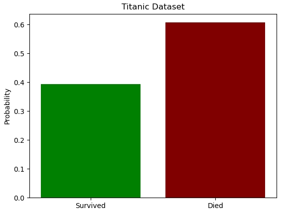
If everyone had survived the titanic, the entropy of the distribution of survived/dead would be zero, since everyone is in the alive class.
If 50% had survived and 50% died, then the entropy would be the maximum possible for 2 classes or
For all other cases, entropy is calculated like this
Where C is the amount of classes
However, the whole point is that we don't know the true q distribution...
That's where cross-entropy comes in.
We can introduce distribution
so our formula becomes
To measure the difference of our distributions
we can use a method called the Kullback-Leibler Divergence
It is a measure of how 'different' two probability distributions are
So as we reach a better approximation of q, the KL divergence will be lower.
This is starting to look more and more like a loss function
During its training, the classifier uses each of the N points in its training set to compute the cross-entropy loss, effectively fitting the distribution p(y)!
The cross-entropy for a set of points is then defined as
However, this is only for a single class, and as we know, our binary classification has 2 classes.
We can further derive a loss function for the two distributions like so:
Where N is the amount of training examples, used to average out the loss.
The terms inside the sum are this way because when we have Yi=1, we only consider cross-entropy on class 'alive' and if we have Yi=0, we only consider it on the class 'dead'.
Now that we understand cross-entropy, let's go back to our neural network.
As mentioned above, due to the problem size, we can use a small neural network to solve it reasonably well.
net = NN(layers=[
	Layer(7, 15, activation='relu'),
	Layer(15, 1, activation='sigmoid'),
], loss='binary_crossentropy', optimizer=SGD())
We have 2 layers, (that's excluding input), one hidden and an output layer with just a single neuron.
Our input layer consists of 7 neurons because of the size of our data
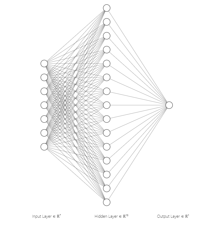
(the visualisation was produced using NN-SVG)
The next step is to prepare the data for modelling, loading it from the csv file from the kaggle competition
np_raw = titanic_data.load_train_data()

X_train = np_raw[:600]

Y_train = X_train[:, 0]

X_train = X_train[:, 1:]
(the titanic_data file will be provided with the article, along with all of the code)
Now we only need to train the network, which is as simple as
net.fit(X_train, Y_train, epochs=1000, learning_rate=0.001, sample_size=150)
Just a little bit more :))
To perform backpropagation and minimize our cost function, we first have to see what goes into calculating it. That's best visualized using a computation graph
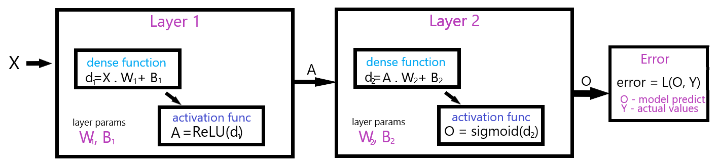
This is how the value of X gets transformed throughout the layers. Our goal is, as in the linear regression example, to optimize our W and B values. However, this time it's a bit more tricky, because our computation chain is longer.
From X to error, the composition of functions is then as follows.
The gradient of the error with respect to the W and B values will then take a bit more to mathematically work out. We can trace the computations back and use the chain rule of differentiation to compute the partial derivatives of both the weights and biases.
For Layer 2:
For Layer 1
Note that the computations here include the computations from Layer 2, because a small change to W1 also cascades into the output of Layer 2
We can expand on the terms from Layer 1 and get
And
As we can see, a lot of the functionality for calculating a layer's W and B partial derivatives can be generalized.
Each layer computes the activation error with respect to its own activation function and with respect to its own dense function.
So lets try to put it into a generalized implementation
We iterate backwards from the final layer to the first one, computing and propagating the error throughout the layers
Where dense_function_w and dense_function_b are the partial derivatives of the linear dense activation function of the layer, with respect to either w or b.
error_or_w is the derivative with respect to the error (in case of the final layer) or with respect to the weight (all other layers).
Then we perform weight / bias updates like this
And finally, we compute the error with respect to this error, which will be later input as error_or_w for the previous layer. (remember, we're going backwards)
Where Wl is this layer's weight.
The python implementation for the layer specific backprop:
Layer Class
    def backward(self, w_or_error, learning_rate, t):
        activation_error = self.compute_activation_error(w_or_error)

        weights_error = np.dot(self.input, activation_error) * (1 / self.N)
        bias_error = np.mean(activation_error, axis=0, keepdims=True)

        self.W, self.B = self.optimizer.step(
            learning_rate,
            weights_error,
            bias_error,
            self.W,
            self.B,
            t
        )

        # compute the error with respect to this layer
        error = np.dot(activation_error, self.W.T)

        return error

    def compute_activation_error(self, w_or_error):
        if self.activation == 'relu':
            return mlmath.relu_derivative(self.D) * w_or_error
        if self.activation == 'sigmoid':
            return mlmath.sigmoid_derivative(self.D) * w_or_error
        if self.activation == 'softmax':
            return w_or_error
        else:
            return w_or_error
This implementation can theoretically work on any number of layers.
The only other part we need is the NN functionality, which enables the backpropagation for all the layers.
NN Class
    def compute_loss_derivative(self, Y_hat, Y):
        if self.loss == 'mse':
            return mlmath.mse_derivative(Y_hat, Y)
        if self.loss == 'binary_crossentropy':
            return mlmath.binary_crossentropy_derivative(Y_hat, Y)
        else:
            return mlmath.batch_error_softmax_input(Y_hat, Y)

    def compute_error(self, Y_hat, Y):
        if self.loss == 'mse':
            return mlmath.mse(Y_hat, Y)
        if self.loss == 'binary_crossentropy':
            return mlmath.binary_crossentropy(Y_hat, Y)
        else:
            return mlmath.cross_entropy(Y_hat, Y)

 def sample(self, x_train, sample_size, y_train):
        indices = np.random.choice(x_train.shape[0], sample_size, replace=False)

        sample_X = x_train[indices]
        sample_Y = y_train[indices]
        return sample_X, sample_Y

    def fit(self, x_train, y_train, epochs, learning_rate, sample_size, include_logs=True):
        n_weight_updates = int(np.ceil(x_train.shape[0] / sample_size))
        t = 1
        for i in range(epochs):
            err = []
            for j in range(n_weight_updates):
                # random sample for minibatch j
                sample_X, sample_Y = self.sample(x_train, sample_size, y_train)

                output = self.predict_(sample_X).T

                # calculate loss derivative
                error = self.compute_loss_derivative(output, sample_Y).T

                # backward propagation
                for layer in reversed(self.layers):
                    error = layer.backward(error, learning_rate, t)
                t += 1
                # calculate average error on all samples
                total_err = self.compute_error(output, sample_Y).T
                err.append(total_err)
            if include_logs:
                print('epoch %d/%d err: %f' % (i + 1, epochs, np.mean(np.array(err))))
A noteworthy thing here: the sample_size parameter is used, because our implementation works with SGD by default.
Stochastic Gradient Descent (SGD) is an optimizer algorithm, used to accelerate convergence. The term 'stochastic' means random, and in the case of plain SGD, that is used to mean a ranom sample of the entire dataset. If we consider a dataset with N = 100000 records, we can imagine that each epoch iteration (optimization) will be really slow. With plain SGD, we can define J to equal any number of examples to randomly sample from the training set and use to make our gradient step. That means that if J=1000, for each epoch, we'll only be iterating over 1000 randomly sampled examples, greatly optimizing the speed.
Plain SGD however takes more steps to converge, due to the fact that we're doing 1 gradient step per epoch and only considering J elements. That is why our implementation will be using Minibatch SGD. Given J=1000, Minibatch SGD will take 100 minibatches for each epoch and it will perform N / J gradient updates each epoch. This helps by reducing the amount of steps SGD needs to converge.
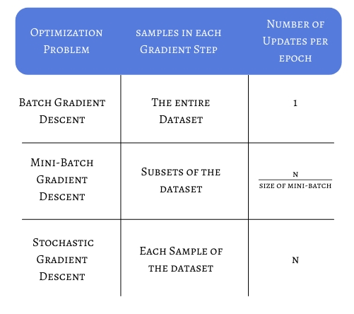
in our implementation, we compute the numbers of updates per epoch like this:
n_weight_updates = int(np.ceil(x_train.shape[0] / sample_size))
Now that's pretty much all we need for our neural network to work!
Let's see it in action with the titanic dataset.
Running the Neural network example from above for 20 experiments, we get these results:
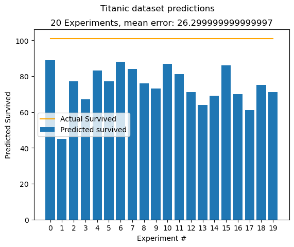
We use the first 600 records to train the algorithm and the rest 281 to measure the performance. We can expect to get a mean error of around 25-30. That is, for how many people in the test set our algorithm was off. I.e predicted survived, but was dead. This is not an objective optimization measure, it is simply used for illustration. We know that in our test set 101 people survived, hence the 101 - mean calculation.
We get a decent result, however improvements can be made :)
ADAM stands for adaptive moment estimation. Yes, i was also disappointed that it was not created by an Adam, who named it after himself. Adam builds upon two already established optimizers, namely
- AdaGrad, which maintains a per-parameter learning rate, which helps with sparse gradients
- RMSProp, which also maintains a per-parameter learning rate, adapted based on the average of recent magnitudes.
The algorithm works by computing an exponential moving average and a squared moving average of the w and b gradients. Two hyperparameters are defined, beta1 and beta2, which control the moving averages' exponential decay rates.
The first moment moving averages are computed as:
And the second moment:
Since the moving averages are initialized as 0s (or vectors of 0s), the moving average will be biased towards 0.
To counter that, the ADAM authors cleverly compute
And for the second moment:
The term in the denominator
is of power t, because this is meant to solve the discrepancy between all time steps up until this point.
The python implementation is relatively straightforward:
class Adam(Optimizer):
    def __init__(self, b1=0.9, b2=0.999, epsilon=1e-8):
        self.b1 = b1
        self.b2 = b2
        self.epsilon = epsilon
        self.m_dw, self.v_dw = 0, 0  # will get transformed to vectors
        self.m_db, self.v_db = 0, 0

  def step(self, learning_rate, dw, db, w, b, t):
        self.m_dw = self.b1 * self.m_dw + (1 - self.b1) * dw
        self.v_dw = self.b2 * self.v_dw + (1 - self.b2) * dw ** 2

        self.m_db = self.b1 * self.m_db + (1 - self.b1) * db
        self.v_db = self.b2 * self.v_db + (1 - self.b2) * db ** 2

        mt_w_hat = self.m_dw / (1 - self.b1 ** t)
        mt_b_hat = self.m_db / (1 - self.b1 ** t)

        vt_w_hat = self.v_dw / (1 - self.b2 ** t)
        vt_b_hat = self.v_db / (1 - self.b2 ** t)

        n_w = w - learning_rate * mt_w_hat / (np.sqrt(vt_w_hat) + self.epsilon)
        n_b = b - learning_rate * mt_b_hat / (np.sqrt(vt_b_hat) + self.epsilon)

        return n_w, n_b
net = NN(layers=[
Layer(7, 15, activation='relu', kernel_initializer=XavierInitializer(7, 15)),
Layer(15, 1, activation='sigmoid', kernel_initializer=XavierInitializer(15, 1)),
], loss='binary_crossentropy', optimizer=Adam())
net.fit(X_train, Y_train, epochs=1000, learning_rate=0.02, sample_size=100, include_logs=False)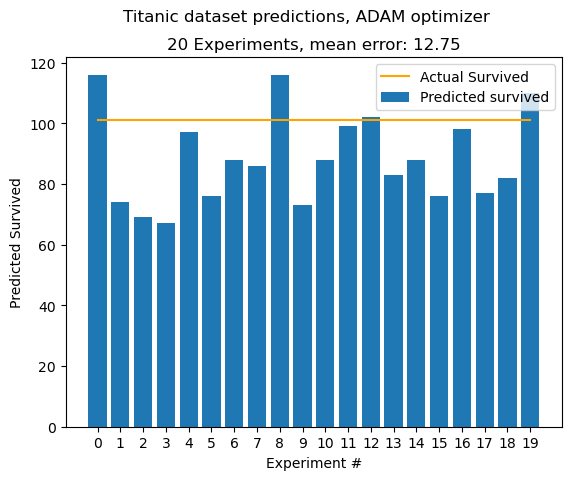
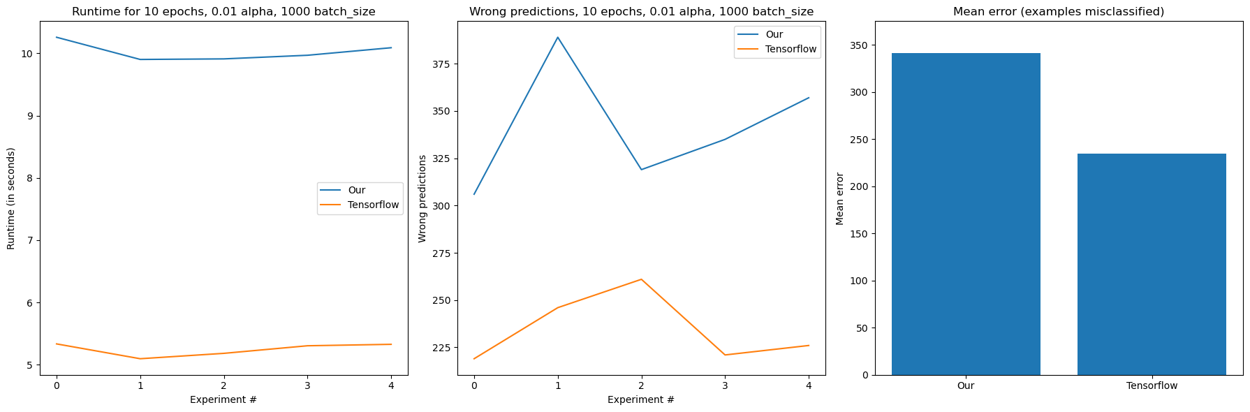
Applying our new optimizer, we can get much better results
So far we have only been computing our gradients on the CPU. This is not that bad of an idea when we're dealing with smaller datasets, however if we try to model something like the MNIST dataset, we'll find that our implementation is still slow:
start = time.time() * 1000

net = NN(layers=[
    Layer(784, 512, activation='relu'),
    Layer(512, 128, activation='relu'),
    Layer(128, 64, activation='relu'),
    Layer(64, 10, activation='softmax'),
], loss='categorical_crossentropy', optimizer=Adam())

net.fit(x_train_flattened, y_train_oh, 10, 0.01, sample_size=1000)
time_n = (time.time() * 1000) - start
print("Time: ", time_n, " ms")
epoch 1/10 err: 4.081437
epoch 2/10 err: 0.318554
...
epoch 9/10 err: 0.047872
epoch 10/10 err: 0.037808
Time: 33409.406494140625 ms
On my machine, which still has a respectable Intel(R) Core(TM) i7-10750H CPU with 6 cores, it takes more than 30 seconds to do 10 epochs of the MNIST dataset. That's because it is gigantic in comparison with the titanic dataset. It features 60000 training images with 28x28 pixels each. If we flatten the pixels that's 60000 vectors with 784 numbers each.
Our NN model isn't shy either, having almost half a million trainable parameters!
And that's nothing in comparison to most real-world datasets.
Fortunately, machine learning algorithms can also make use of the graphics processor, which was idling up until this point.
The GPU is designed to work super well for graphics computations, which luckily, are essentially linear algebra and therefore matrix multiplication.
The developers at NVIDIA know this and have been maintaining a platform to interface with the graphics processor for non-graphics, parallel computations, called CUDA. And there also exists a numpy abstraction, which can perform all arithmetic using CUDA and on the GPU, called CuPy
Setting up CuPy with all of its dependencies can be tedious, the guide i followed is this one
Once set up, CuPy is relatively straightforward to use as almost all CuPy functions are 1:1 identical with their numpy counterparts. Some things in mind however:
- CuPy Arrays are not interchangeable with numpy arrays.They still use ndarray, however the implementation is different. Explicit conversion is needed between the two
- Overhead: This solution introduces a lot of overhead as it needs to send data to the GPU from the CPU. On datasets such as titanic, there is a huge performance drop
- As mentioned 'almost all' functions are 1:1 equivalent to numpy. Some of the differences are explained here
Let's now try modelling MNIST with CuPy and GPU hardware acceleration:
CUPY NN IMPLEMENTATION
import cupy as cp


import cuda_mlmath
from cuda_initializers import XavierInitializer
from cuda_optimizers import SGD
import copy

import time

class LayerV2:
    def __init__(self, input_size, output_size, activation, kernel_initializer=None):
        self.kernel_initializer = kernel_initializer
        self.optimizer = None
        if kernel_initializer is None:
            self.kernel_initializer = XavierInitializer(input_size, output_size)

        self.activation = activation

        self.W = self.kernel_initializer.W()
        self.B = self.kernel_initializer.B()

    def backward(self, w_or_error, learning_rate, t):
        activation_error = self.compute_activation_error(w_or_error)

        weights_error = cp.multiply(cp.dot(self.input, activation_error), (1 / self.N))

        # Breaks CuDNN if we try to take the mean of (N, 1) matrix with respect to axis 0
        bias_error = cp.mean(activation_error, axis=0, keepdims=True) if activation_error.shape[1] != 1 else cp.mean(activation_error, keepdims=True)

        self.W, self.B = self.optimizer.step(
            learning_rate,
            weights_error,
            bias_error,
            self.W,
            self.B,
            t
        )

        # compute the error with respect to this layer
        error = cp.dot(activation_error, self.W.T)

        return error

    def compute_activation_error(self, w_or_error):
        if self.activation == 'relu':
            return cp.multiply(cuda_mlmath.relu_derivative(self.D), w_or_error)
        if self.activation == 'sigmoid':
            return cp.multiply(cuda_mlmath.sigmoid_derivative(self.D), w_or_error)
        if self.activation == 'softmax':
            return w_or_error
        else:
            return w_or_error

    def dense_pass(self, X):
        return cp.dot(X, self.W) + self.B

    def activation_pass(self, X):
        if self.activation == 'relu':
            return cuda_mlmath.relu(X)
        if self.activation == 'sigmoid':
            return cuda_mlmath.sigmoid(X)
        if self.activation == 'softmax':
            return cuda_mlmath.batch_softmax(X)
        else:
            return X  # linear

    def layer(self, X):
        self.input = X.T
        self.N = X.shape[0]
        D = self.dense_pass(X)
        A = self.activation_pass(D)
        self.D = D
        return A


class NNV2:
    def __init__(self, layers, loss='mse', optimizer=SGD()):
        self.loss = loss
        self.layers = layers
        self.optimizer = optimizer
        for layer in layers:
            layer.optimizer = copy.copy(optimizer)

    def compute_loss_derivative(self, Y_hat, Y):
        if self.loss == 'mse':
            return cuda_mlmath.mse_derivative(Y_hat, Y)
        if self.loss == 'binary_crossentropy':
            return cuda_mlmath.binary_crossentropy_derivative(Y_hat, Y)
        else:
            return cuda_mlmath.batch_error_softmax_input(Y_hat, Y)

    def compute_error(self, Y_hat, Y):
        if self.loss == 'mse':
            return cuda_mlmath.mse(Y_hat, Y)
        if self.loss == 'binary_crossentropy':
            return cuda_mlmath.binary_crossentropy(Y_hat, Y)
        else:
            return cuda_mlmath.cross_entropy(Y_hat, Y)

    def predict(self, X):
        x_pred = cp.array(X) # To keep consistency with V1, we convert to cupy array here
        output = x_pred
        for layer in self.layers:
            output = layer.layer(output)
        output = cp.asnumpy(output) # And output as numpy
        return output

    def predict_(self, X):
        output = X
        for layer in self.layers:
            output = layer.layer(output)
        return output

    def sample(self, x_train, sample_size, y_train):
        indices = cp.random.choice(x_train.shape[0], sample_size, replace=False)

        sample_X = x_train[indices]
        sample_Y = y_train[indices]
        return sample_X, sample_Y

    def fit(self, x_train, y_train, epochs, learning_rate, sample_size, include_logs=True):
        x_train_cp = cp.array(x_train)
        y_train_cp = cp.array(y_train)

        n_weight_updates = int(cp.ceil(x_train_cp.shape[0] / sample_size))
        t = 1
        for i in range(epochs):
            err = []
            for j in range(n_weight_updates):
                # random sample for minibatch j
                sample_X, sample_Y = self.sample(x_train_cp, sample_size, y_train_cp)

                output = self.predict_(sample_X).T

                # calculate loss derivative
                error = self.compute_loss_derivative(output, sample_Y).T

                # backward propagation
                for layer in reversed(self.layers):
                    error = layer.backward(error, learning_rate, t)
                t += 1
                # calculate average error on all samples
                total_err = self.compute_error(output, sample_Y).T
                err.append(total_err)
            if include_logs:
                print('epoch %d/%d err: %f' % (i + 1, epochs, cp.mean(cp.array(err))))
And then model the same dataset:
net = NNV2(layers=[
    LayerV2(784, 512, activation='relu'),
    LayerV2(512, 128, activation='relu'),
    LayerV2(128, 64, activation='relu'),
    LayerV2(64, 10, activation='softmax'),
], loss='categorical_crossentropy', optimizer=Adam())

net.fit(x_train_flattened, y_train_oh, 10, 0.01, sample_size=1000)
time_n = (time.time() * 1000) - start

print("Time: ", time_n, " ms")
epoch 1/10 err: 3.609623
epoch 2/10 err: 0.426479
...
epoch 10/10 err: 0.067483
Time: 10219.15283203125 ms
Other improvements that can (and probably should) be made are:
- Only require a single parameter when creating the layer. It is unnecessary to write them in a pair (N,J) when we know that this layer has N neurons and the next has J
- L1 and L2 regularization
- Accuracy metrics
- The AMSGRAD optimizer, as it is arguably even faster than ADAM
- Ability to store weights in a file
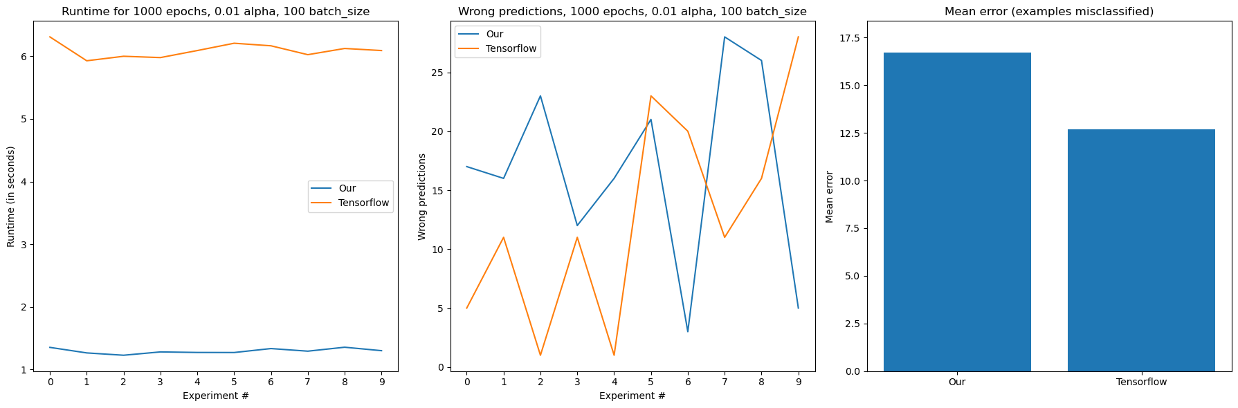
Expecting to outperform tensorflow would be naive, but we gave it a good try :)
The code style for this implementation was inspired by Omar Aflak and his Towards Data Science Article
https://en.wikipedia.org/wiki/Multilayer_perceptron
https://en.wikipedia.org/wiki/Artificial_neural_network
https://www.sciencedirect.com/topics/neuroscience/artificial-neural-network
https://en.wikipedia.org/wiki/Artificial_neuron
https://www.tibco.com/sites/tibco/files/media_entity/2021-05/neutral-network-diagram.svg
https://en.wikipedia.org/wiki/Multilayer_perceptron
https://en.wikipedia.org/wiki/Convolutional_neural_network
https://en.wikipedia.org/wiki/Recurrent_neural_network
https://en.wikipedia.org/wiki/Graph_neural_network
https://en.wikipedia.org/wiki/Bombay_cat
https://en.wikipedia.org/wiki/Theory_of_forms
https://www.cuemath.com/calculus/linear-functions/
https://en.wikipedia.org/wiki/Simple_linear_regression
https://www.kaggle.com/code/prasadperera/the-boston-housing-dataset
https://en.wikipedia.org/wiki/Mean_squared_error
https://en.wikipedia.org/wiki/Gradient
https://en.wikipedia.org/wiki/Partial_derivative
https://en.wikipedia.org/wiki/Gradient
https://en.wikipedia.org/wiki/Gradient_descent
https://news.mit.edu/2017/explained-neural-networks-deep-learning-0414
https://aws.amazon.com/what-is/overfitting/
https://www.tensorflow.org/guide/keras/sequential_model
https://en.wikipedia.org/wiki/Sigmoid_function
https://en.wikipedia.org/wiki/Rectifier_%28neural_networks%29
https://www.learndatasci.com/glossary/sigmoid-function/
https://en.wikipedia.org/wiki/Softmax_function
https://cs230.stanford.edu/section/4/
https://www.kaggle.com/c/titanic
https://en.wikipedia.org/wiki/Random_forest
https://en.wikipedia.org/wiki/XGBoost
https://en.wikipedia.org/wiki/Kullback%E2%80%93Leibler_divergence
http://alexlenail.me/NN-SVG/index.html
https://www.kaggle.com/c/titanic
https://s12.gifyu.com/images/ezgif.com-video-to-gif0a780b1f48281f55.gif
https://www.tutorialspoint.com/python_deep_learning/python_deep_learning_computational_graphs.htm
https://en.wikipedia.org/wiki/Chain_rule
https://www.baeldung.com/cs/mini-batch-vs-single-batch-training-data
https://arxiv.org/pdf/1412.6980.pdf
https://machinelearningmastery.com/adam-optimization-algorithm-for-deep-learning/
https://en.wikipedia.org/wiki/MNIST_database
https://en.wikipedia.org/wiki/CUDA
https://docs.cupy.dev/en/stable/index.html
https://docs.cupy.dev/en/stable/install.html#installing-cupy
https://docs.cupy.dev/en/stable/user_guide/difference.html
https://towardsdatascience.com/l1-and-l2-regularization-methods-ce25e7fc831c
https://arxiv.org/pdf/1904.09237.pdf
https://towardsdatascience.com/math-neural-network-from-scratch-in-python-d6da9f29ce65